From crystals to market making: an overview of legendre - part 1

When I was doing my studies for my doctorate, there was one course I found immediately interesting: “classical condensed matter”. If that doesn’t mean anything to you that’s fine. It boils down to understanding the behaviour of materials like glasses and ice at a reasonably high level, meaning at the scale you could maybe get to with a run-of-the-mill optical microscope. I mention this because the focus of most of my physics research was at several orders of magnitude smaller scales in both space and time, so this was refreshing to study things at a much higher level, literally.

The most interesting part of the class was when we started getting to alloys and metallurgy. The amount of physics required to understand concepts like impingement and diffusion under stress, for example, was mindboggling, and very cool. A large portion of the class was dedicated to the concept of “if you can’t teach it you don’t understand it”, and part of that Socratic method was programming: simulating the equations and physics you learn so you can be forced to confront the equations you most likely have no hope of understanding (at least in the beginning).

Part of this was what we came to learn as “Model C”, a particular so-called phase-field model that tries to understand the dynamics of interfacial problems. Interfacial here means that we want to figure out how a material (here represented by a field $\varphi$) evolves in its environment. A simple example of an interfacial problem is tracking the sonic boom that the bald eagle makes in the USPS logo as it soars through the skies (I’m not kidding, apparently this eagle breaks almost to Mach 5).

In my case, though, it’s not the fastest bird alive that I was interested in. It was nucleation and crystal growth, specifically dendrites. These are the “fingers” that grow — think like the tails of a snowflake — when a material crystallizes in some ambient environment. The model itself is actually one of the seminal models of the field, from Karma & Rappel, PRE 57, 4323 (1998). It breaks down to two coupled fields that together constitute a set of partial differential equations describing how the phase field $\varphi$ evolves over time, relative to the heat field $u$:

The most interesting piece to me, though, was that this model also has anisotropy in the surface tension, meaning that the rate of growth of the tip of the dendrite in one direction is not the same as that in another, which results in uneven crystal growth. This boils down to 4-fold anisotropy $A(\theta) = \bar{a}(1 + \varepsilon^\prime \cos 4\theta)$, relaxation time $\tau(\mathbf{n}) = A(\mathbf{n})^2$, thermal diffusivity $D = a_2 \lambda$, and mirror (no-flux) boundaries.

All of this to say, though, is that there was this KILLER equation to solve, and some beautiful crystals to grow, so how do we do this??

At the time, I used Fortran and just brute forced the hell out of the equations, because I was focusing more on the physics than the programming. Let me tell you, it results in some lovely code:

    REAL(dp) :: DERX_r, DERX_l, DERX_t, DERX_b, DERY_t, DERY_r, DERY_l, DERY_b
    REAL(dp) :: MAG2_R, A_R, dA_R, MAG2_L, A_L, dA_L, MAG2_T, A_T, dA_T, MAG2_B, A_B, dA_B
    REAL(dp) :: DERX, DERY, MAG2, A, JR, JL, JT, JB
    REAL(dp) :: g_prime, h_prime, P_prime, noise

    CALL MPI_Init ( ierr )
    call MPI_Comm_rank ( MPI_COMM_WORLD, myrank, ierr )
    call MPI_Comm_size ( MPI_COMM_WORLD, nprocs, ierr )
    wtime = MPI_Wtime( )

    WRITE(6, '(5x, a21)', advance="no") "Allocating arrays ..."
    ...
    !$omp parallel do schedule(guided) default(shared) private(i, j)
        DO i = 2, N+1
            DO j = 2, N+1
                !define derivative on edges of finite volume in x
                DERX_r = phi(i+1,j)-phi(i,j); DERX_l = phi(i,j)-phi(i-1,j)
                DERX_t = 0.25*(phi(i+1,j+1)-phi(i-1,j+1)+phi(i+1,j)-phi(i-1,j))
                DERX_b = 0.25*(phi(i+1,j)-phi(i-1,j)+phi(i+1,j-1)-phi(i-1,j-1))
                ...
            ENDDO !x
        ENDDO !y
    !$omp end parallel do

But now, looking back on this, I wanted to do better. Much better. So much better, in fact, that the solution I decided to build breaks through being able to simulate crystals, and really ended up taking on a life of its own as a full-fledged PDE framework, lovingly called legendre.

What is it?

legendre is a block-structured, deterministic, scheduler-driven framework for time-dependent PDEs — the kind you can write as a method-of-lines system:

deterministic or stochastic, in any spatial dimension. Model C is one model you can hand it. So is the 3D heat equation, which is about sixty lines. The framework is not “a dendrite solver” — the dendrite solver is a client of it.

The thesis, and the thing my Fortran got catastrophically wrong, is one sentence: the mathematics, the numerics, and the execution are three different concerns, and they should not know about each other. My Fortran welded all three into a single triple-nested loop — the physics, the finite-volume stencil, the OpenMP schedule, and the MPI halo exchange all braided through the same fifty lines. Change any one and you re-derive all four. legendre pulls them apart, and then lets the type system hold them apart.

Four rules the compiler enforces

The whole design is four rules, and the point is that they aren’t style guidelines you can quietly violate on a deadline — they’re baked into trait signatures, so violating them doesn’t compile:

1. Mathematical objects own no execution. A Model cannot spawn a thread. A Grid cannot open a file. An Operator cannot allocate. If a trait’s job is mathematics, its signature has no way to express a side effect — there’s no scheduler in scope to abuse.
2. Execution is scheduler-driven. Exactly one module in the crate is allowed to say the word Rayon. A SerialScheduler is the oracle, and every parallel scheduler has to reproduce it bit for bit — a test asserts exactly that.
3. Storage is separate from views. An Allocator hands out opaque byte slabs exactly once, at setup. Everything the solver touches afterward is a typed, ghost-aware view into those bytes. Nothing allocates in the hot loop.
4. Numerics are policies. Grid + Discretization → Operators. A model states what operator it needs; it never learns how that operator was built.

That fourth one is what makes the whole thing sing, so let’s dwell on it.

Models say what, schemes say how

Here is the signature that does the heavy lifting. A diffusion model needs a Laplacian. It says exactly that, and nothing more:

impl<G, D> Model<G, D> for Diffusion
where
    D: Discretizes<G, Laplacian>,   
{
    // rhs reads ∇²u through an operator it never had to build,
    // on a grid whose dimension it never had to name.
}

Diffusion has no idea whether its Laplacian is second-order finite differences on a Cartesian grid, a finite-volume flux divergence, or something coarse–fine-aware running under adaptive refinement. It asked for a Laplacian; it got one. Which means swapping the numerical method is a one-line change in the wiring, with zero edits to the physics:

let mut sim = Simulation::new(
    grid,
    FiniteDifference,   // central, 2nd order
    FiniteVolume,       // Karma–Rappel anisotropic flux
    model, integrator, scheduler, allocator,
);

Dimension gets the same treatment: it’s an associated const D: usize on the concrete grid, not something generic solver code ever touches. The 2D and 3D heat models in the repo are the same source text — you write Heat::<2> or Heat::<3> and the framework does the rest.

The timestep, and a bug you’re not allowed to write

Model::step() does not exist. This is deliberate, and it’s one of my favourite decisions in the codebase. A model exposes its right-hand side — dY/dt — and is forbidden from mutating state or even seeing dt. The integrator owns the update. That single boundary is what makes multi-stage schemes fall out for free: RK4 is about forty lines of pure vector algebra, because every stage buffer is slab-congruent with the state and the integrator just does axpy.

And because the integrator owns dt, it also owns the √dt that stochastic terms need. The model provides driver-indexed vector fields,

and the model’s set of noise drivers is a type — NoNoise or Wiener<M>. Two classic hand-rolled-solver bugs become literally inexpressible. Scaling the noise by dt instead of √dt? You can’t — the model never touches dt, and the integrator applies the correct power. Running a stochastic model with a deterministic-only scheme? RungeKutta4 implements Integrator<G, D, NoNoise> and nothing else, so:

// ModelC drives a Wiener process (its sidebranching noise).
let sim = Simulation::new(grid, FiniteVolume, ModelC::new(),
    RungeKutta4, RayonScheduler, SystemAllocator);
// error[E0277]: the trait bound `RungeKutta4: Integrator<_, _, Wiener<_>>`
//               is not satisfied

Reach for EulerMaruyama instead and it compiles. The type system caught a subtle numerical-methods mistake at the wiring stage, before a single cell was ever updated.

The block is the atom, not the grid

Underneath all of this, the fundamental unit isn’t the grid — it’s the block. Even a uniform Cartesian grid is just a tiling of congruent blocks, each carrying a ghost ring halo-exchanged from its neighbours (or filled by the model’s boundary conditions):

Grid                    one Block (ghost-inclusive slab)
┌────┬────┬────┐        ╔═══════════════════╗
│ B0 │ B1 │ B2 │        ║ g  g  g  g  g  g  ║   g = ghost ring
├────┼────┼────┤        ║ g ┌─────────────┐ ║       (from neighbours, or from
│ B3 │ B4 │ B5 │  ───►  ║ g │  interior   │ ║        the model's boundary
├────┼────┼────┤        ║ g │  cells      │ ║        conditions on real edges)
│ B6 │ B7 │ B8 │        ║ g └─────────────┘ ║
└────┴────┴────┘        ╚═══════════════════╝

That one decision pays for itself several times over. State is stored block-major, so the scheduler hands each worker a structurally disjoint &mut BlockStorage — genuinely parallel mutation with no interior mutability and no unsafe, because the borrow checker can see the blocks don’t overlap. And adaptive mesh refinement becomes invisible to the execution model: refinement just replaces one block with children, and the scheduler never notices. The AMR grid runs behind the exact same Grid trait as the uniform one.

Determinism is a constraint, not an aspiration

Reproducibility in a parallel stochastic solver is usually a punchline. Here it’s a hard guarantee, and it comes from two decisions. Block writes are disjoint and land at fixed slab locations, so the order the scheduler happens to visit blocks in cannot change the answer — the suite asserts serial and Rayon runs are bitwise identical, including the stochastic ones. And there is no RNG stream to advance, which is the usual source of order-dependence. Every random increment is a pure function

via a SplitMix64 chain into Box–Muller. Any thread count, any visitation order: identical noise. To reproduce a run — the whole run, a hundred million cells and all — you need its seed. That’s the entire reproduction recipe.

A toy example: heat in three dimensions

Alright so let’s actually do something. Building a simulation is picking one type from each column — grid, discretization, model, integrator, scheduler, allocator — and letting them compose:

let grid = CartesianGrid::new([96; 3], [32; 3], [0.0; 3], [0.1; 3])?;
let mut sim = Simulation::new(
    grid, FiniteDifference, Heat::<3> { kappa: 0.7, u: None },
    ForwardEuler, RayonScheduler, SystemAllocator,
);

let dt = sim.stable_dt().unwrap();
for _ in 0..steps { sim.step(dt); }

Defining the Heat model itself is three methods — register_fields (what fields exist), fill_ghosts (halos and boundary conditions), and vector_field_block (the actual right-hand side). Everything else — the parallelism, the stage buffers, the output — is wiring you never write:

impl<const D: usize, G, Disc> Model<G, Disc> for Heat<D>
where Disc: Discretizes<G, Laplacian>
{
    fn register_fields(&self, /* … */) { /* one field: u */ }
    fn fill_ghosts(&self, /* … */)     { /* mirror BCs on the faces */ }
    fn vector_field_block(&self, /* … */) {
        // du/dt = κ ∇²u   — that is the physics, all of it
    }
}

Growing a crystal

Which brings us back to the dendrites. The shipped ModelC is exactly the Karma–Rappel solidification model from the top of this post — coupled φ/u, four-fold anisotropy, multi-grain nucleation with a per-grain crystallographic orientation baked in as a static Voronoi field. You run it like anything else:

$ cargo run --release --example model_c
⠁ [00:01:12] ████████████░░░░░░░░ 45231/187000 (628 steps/s, eta 3m 46s)
  t=723.7 | phi∈[-1.00,1.00] ⟨phi⟩=-0.53 frac>0: 23.4% | u∈[-0.70,0.09] ⟨u⟩=-0.512

A 210² grid for 25,000 steps finishes in seven or eight seconds — about 7 nanoseconds per cell-step, snapshots included. Turn it up and it goes to 101.6 million cells (a 10080² domain tiled as 80×80 blocks of 126² each), a thousand grains with random orientations, at ~12 GB peak — and nothing allocates after Simulation::new. The field storage, the stage buffers, the worker-pinned scratch, and the snapshot ring are all built once:

RUSTFLAGS="-C target-cpu=native" cargo build --profile maxperf --example model_c
./target/maxperf/examples/model_c --cells 10080 --block 126 \
    --seeds 1000 --orient --noise 0.02 --time 350 --every 4000 --ring 2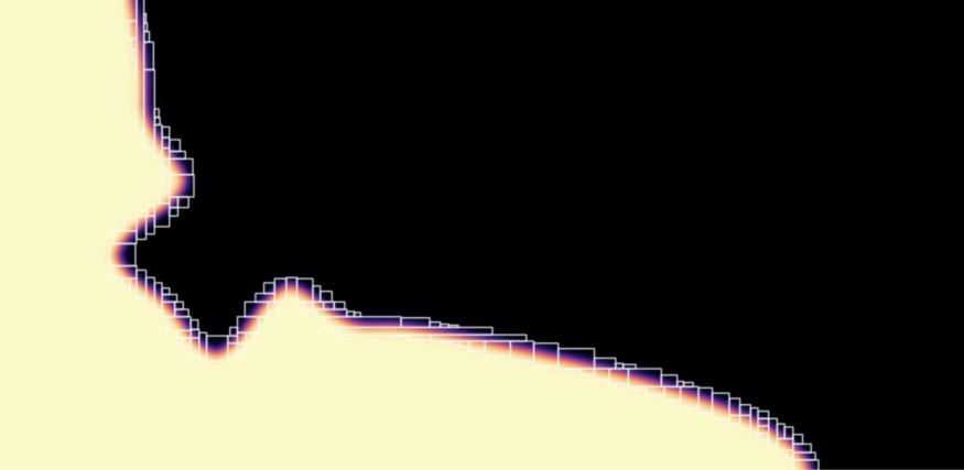

And when you’re lucky enough, you get my favourite results: this beautiful dendrite growing across a glowing interface into an undercooled melt. Worth it!

The reading

My Fortran solved exactly one equation and could never solve another, because the equation, the scheme, the threads, and the message-passing were all the same forty lines. The moment I wanted a different crystal — let alone a different field entirely — I’d have started over.

legendre’s bet is that if you refuse to let the mathematics know how it’s being computed, the mathematics outlives the machine. The physics is sixty lines that never mention a thread; the parallelism is one module that never mentions physics; and a SerialScheduler stands behind all of it as a bitwise oracle proving the fast path didn’t lie. The design rationale even lives as doc comments on the traits themselves — the one place, as I’ve painfully learned, where documentation can’t rot away from the code it describes.

If you can’t teach it, you don’t understand it. It turns out the same is true of code: if you can’t cleanly separate what you’re computing from how, you probably never understood either one.

Part 2 shows how this engine can do some much more stunning things with the same framework, so stay tuned.